# Prediction grid
temp_range <- seq(-5, 35, by = 0.5)
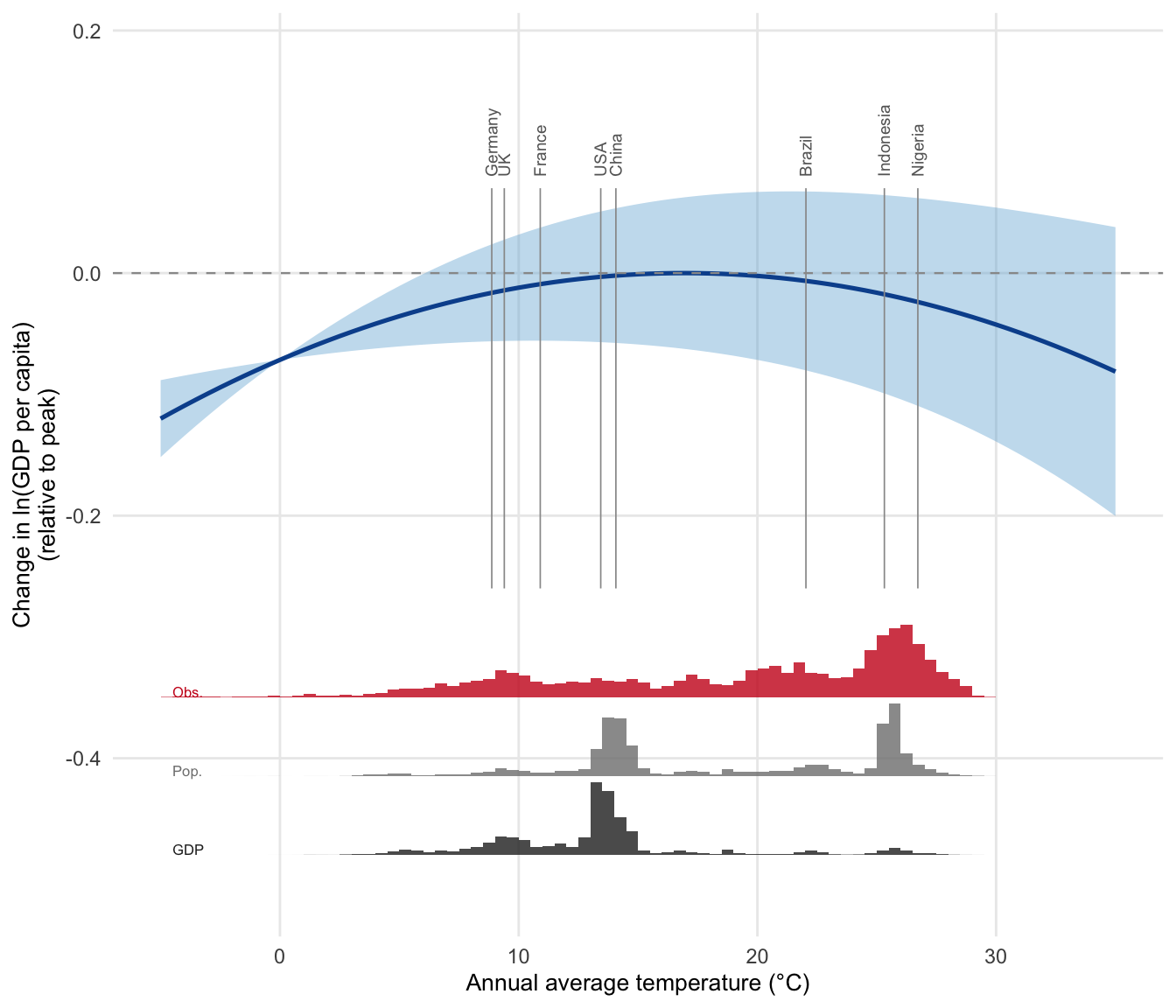
# Predicted growth (linear + quadratic terms)
y_hat <- b1 * temp_range + b2 * temp_range^2
# Delta-method standard errors: SE(ŷ) = sqrt(X' Var(β) X)
vcov_mat <- vcov(model_main)[c("UDel_temp_popweight", "temp_sq"),
c("UDel_temp_popweight", "temp_sq")]
se_fit <- sapply(temp_range, function(t) {
x <- c(t, t^2)
sqrt(as.numeric(t(x) %*% vcov_mat %*% x))
})
# Center predictions at the maximum
y_center <- y_hat - max(y_hat)
ci_lower <- y_hat - 1.96 * se_fit - max(y_hat)
ci_upper <- y_hat + 1.96 * se_fit - max(y_hat)
pred_df <- data.frame(
temp = temp_range,
y = y_center,
ci_lower = ci_lower,
ci_upper = ci_upper
)
# Histogram data (0.5°C bins)
bins <- seq(-6, 30, by = 0.5)
bin_mids <- bins[-length(bins)] + 0.25
hist_temp <- bhm_data$UDel_temp_popweight
hist_pop <- bhm_data$Pop
hist_gdp <- bhm_data$TotGDP
n_bins <- length(bins) - 1
pop_by_bin <- numeric(n_bins)
gdp_by_bin <- numeric(n_bins)
count_by_bin <- numeric(n_bins)
for (j in seq_len(n_bins)) {
in_bin <- hist_temp >= bins[j] & hist_temp < bins[j + 1]
count_by_bin[j] <- sum(in_bin)
pop_by_bin[j] <- sum(hist_pop[in_bin], na.rm = TRUE)
gdp_by_bin[j] <- sum(hist_gdp[in_bin], na.rm = TRUE)
}
# Normalize
scale_factor <- 0.06
count_norm <- count_by_bin / max(count_by_bin) * scale_factor
pop_norm <- pop_by_bin / max(pop_by_bin) * scale_factor
gdp_norm <- gdp_by_bin / max(gdp_by_bin) * scale_factor
base_y <- -0.35
spacing <- 0.065
hist_df <- data.frame(
xmin = bins[-length(bins)],
xmax = bins[-1],
temp_h = base_y,
temp_t = base_y + count_norm,
pop_h = base_y - spacing,
pop_t = base_y - spacing + pop_norm,
gdp_h = base_y - 2 * spacing,
gdp_t = base_y - 2 * spacing + gdp_norm
)
# Country reference lines
selected <- data.frame(
iso = c("DEU", "USA", "NGA", "IDN", "GBR", "FRA", "CHN", "BRA"),
label = c("Germany", "USA", "Nigeria", "Indonesia", "UK", "France", "China", "Brazil")
)
country_temps <- bhm_data %>%
filter(iso %in% selected$iso) %>%
group_by(iso) %>%
summarise(mean_temp = mean(UDel_temp_popweight, na.rm = TRUE)) %>%
left_join(selected, by = "iso")
ggplot() +
# CI ribbon
geom_ribbon(data = pred_df,
aes(x = temp, ymin = ci_lower, ymax = ci_upper),
fill = "#6BAED6", alpha = 0.4) +
# Response curve
geom_line(data = pred_df,
aes(x = temp, y = y),
color = "#08519C", linewidth = 0.9) +
# Zero reference line
geom_hline(yintercept = 0, linetype = "dashed", color = "gray60", linewidth = 0.4) +
# Country vertical lines
geom_segment(data = country_temps,
aes(x = mean_temp, xend = mean_temp, y = -0.26, yend = 0.07),
color = "gray60", linewidth = 0.3) +
geom_text(data = country_temps,
aes(x = mean_temp, y = 0.08, label = label),
angle = 90, hjust = 0, size = 2.5, color = "gray40") +
# Temperature histogram (red)
geom_rect(data = hist_df,
aes(xmin = xmin, xmax = xmax, ymin = temp_h, ymax = temp_t),
fill = "#CB181D", color = NA, alpha = 0.8) +
# Population histogram (gray)
geom_rect(data = hist_df,
aes(xmin = xmin, xmax = xmax, ymin = pop_h, ymax = pop_t),
fill = "gray50", color = NA, alpha = 0.8) +
# GDP histogram (black)
geom_rect(data = hist_df,
aes(xmin = xmin, xmax = xmax, ymin = gdp_h, ymax = gdp_t),
fill = "gray15", color = NA, alpha = 0.8) +
annotate("text", x = -4.5, y = base_y + 0.005, label = "Obs.", hjust = 0, size = 2.2, color = "#CB181D") +
annotate("text", x = -4.5, y = base_y - spacing + 0.005, label = "Pop.", hjust = 0, size = 2.2, color = "gray50") +
annotate("text", x = -4.5, y = base_y - 2*spacing + 0.005, label = "GDP", hjust = 0, size = 2.2, color = "gray15") +
scale_x_continuous(limits = c(-5, 35),
breaks = seq(0, 30, by = 10),
name = "Annual average temperature (°C)") +
scale_y_continuous(name = "Change in ln(GDP per capita)\n(relative to peak)",
limits = c(base_y - 2.5 * spacing, 0.18)) +
theme_minimal(base_size = 11) +
theme(
panel.grid.minor = element_blank(),
axis.title = element_text(size = 10),
plot.caption = element_text(size = 8, color = "gray50")
)